Introduction
Supply and demand are the two fundamental components of a market. Supply describes how producers and manufacturers, large or small, react or behave in the marketplace when producing and selling a product. An understanding of how factors affected supply situations in the past will help farm managers understand possible supply prospects in the future.
The concept of supply
The word 'supply' is commonly used to mean 2 different things. One definition of supply is the total of new production and stocks. 'Stocks' is the amount of product available at the beginning of a new production period. In other words, supply is the total quantity available. The term 'total supply' will be used to indicate the total quantity available.
The other common use of supply describes how producers react in the marketplace. Market supply or aggregate supply represents the amount of a product all producers are willing to sell over a range of prices at any given time period. At an individual level, a producer may be willing to sell a particular quantity as long as the market price is equal to or greater than the cost of producing that quantity. Market or aggregate supply is the total of the quantities all individual farmers want to bring to market at various price levels.
Market supply is represented graphically as an upward sloping curve or line with price on the vertical axis and quantity on the horizontal axis. An increase in price, in most instances, will result in farmers wanting to increase the quantities they bring to the market, so the relationship between price and supply is positive.
Image 1 shows a typical supply curve or line. It shows that as price increases, producers of the product are willing to produce more.
Image 1. Figure 1, Graph showing typical market supply curve

Supply influences
Factors important in influencing supply actions of producers include:
- the price of the product being supplied
- the number of firms producing the product
- technological advances
- the price of inputs
- the price of other or alternative products that could be produced
- unpredictable events such as the weather
Shifts in supply
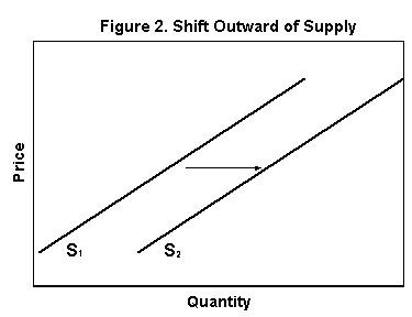
Supply shifts occur because of a change in at least one of the factors listed above, excluding the price of the product itself. A supply shift is a movement of the supply curve at all price levels. A shift outward in supply, shown in Image 2, occurs when producers are willing to produce more of a product at all price levels.
Image 2. Figure 2, Graph showing shift outward of supply curve
The number of firms producing a product affects supply in the same way as the number of consumers (size of population) affects demand: the more firms producing, the greater and more competitive the supply. The opposite also applies – fewer firms generally produce a smaller supply. The size of producers is not strictly the number of firms or farms, but also the size of those farms. The number of farms has been declining over time, but the farmed land base has not changed as much.
Technological advances are an important factor in agriculture supply. Individual people can consume only a limited amount of food, but technology has contributed greatly to the ability of producers to grow more. Technology has been used to improve the performance of almost everything in agriculture, from seeds to livestock to equipment. Over time, the adoption of technology in the production of agricultural products has been a prime factor shifting the supply curve rapidly outward, shown in Image 2. The adoption of technology in agriculture has expanded agricultural output over a range of prices. In other words, applying new technology to agricultural production has lowered costs, so at each price more production is offered for sale.
The price of inputs can also change the position of the supply curve. If the price of inputs declines, it is possible to generate more output without any change in the cost of production. Conversely, if input prices rise, a smaller amount of product can be produced without the farmer paying higher production costs. For example, if the price of fertilizer increases, either less fertilizer is used or total expenditure on inputs must be increased.
The price of alternative products acts on supply in a way similar to how the price of substitutes and complements act on demand. In particular, if the price of a substitute product changes, producers may switch their production decisions. For example, if the price of barley is expected to go up relative to the price of wheat, then producers may alter their cropping patterns to produce more barley and less wheat.
When all production inputs have been committed there are still important random influences on supply, such as weather. Shifts in supply due to weather may be significant and impossible to forecast. Examples of other unpredictable events include ravages by insects and some ad hoc government programs.
Elasticity of supply
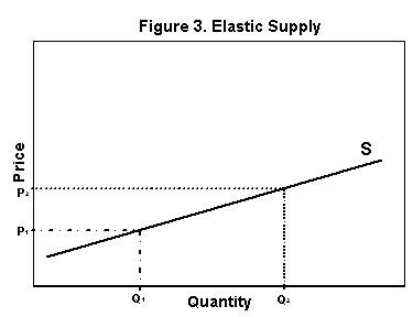
Supply elasticity is a measure of how much producers of a product change the quantities they are willing to sell in response to a change in price. If the change in sales is large compared to a unit change in price, supply is said to be elastic.
Image 3 shows an elastic supply curve. Notice how a relatively small price increase results in a large increase in the amount producers are willing to sell.
Image 3. Figure 3, Graph showing elastic supply curve
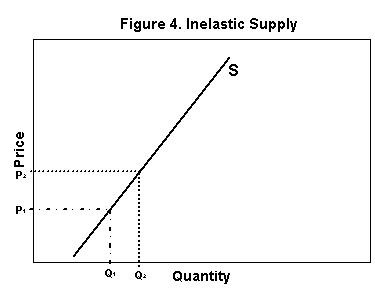
Conversely, if the change in the quantity supplied is small relative to a unit change in price, supply is said to be relatively inelastic.
Image 4 shows an inelastic supply situation, where a price increase does not result in a large increase in the amount that producers are willing to sell.
Image 4. Figure 4, Graph showing inelastic supply curve
Supply elasticity is usually written as a positive number since a higher price can be expected to result in more product being offered for sale and a smaller price will usually result in less product offered for sale.
It is important to understand the difference between shifts in supply and changes in quantity supplied. Shifts in supply occur as a result of a change in one or more of the supply influences but not a change in the product's price. A supply shift changes the amount producers are willing to supply at all price levels. Changes in quantity supplied occur only as a result of a change in the price of the product. A change in quantity supplied is represented as a change in position along a product's supply curve with all other factors staying the same.
Several factors have an influence on the quantity supplied in response to a product's price changes. The factors include:
- time
- the cost structure of producers
- producer price expectations
- ability to store a product
- the ease of changing from the production of one product to another
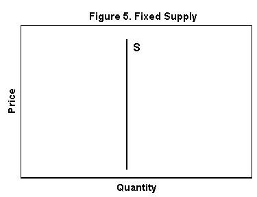
The influence of time may be short, medium or long-term. In the short-term, responsiveness of quantity supplied to price change tends to be small as changes cannot be made quickly. Once a crop is seeded, for example, farmers have limited ability to alter the quantities they put on the market. Therefore, in the short-term, market supply is relatively inelastic or unresponsive. Where there is no opportunity to adjust production in response to price, the supply curve is vertical and the market supply is fixed.
Image 5 shows a fixed supply curve where, regardless of price, quantity supplied or market supply remains constant. As the length of time represented in the supply curve – the production time period – grows, market supply tends to become more elastic or more responsive to price changes.
Image 5. Figure 5, Graph showing fixed supply curve
The physical production process of any particular commodity influences how much time must pass for a term to be considered short or long. The short-term is that length of time over which only a few inputs can be changed. For example, once land is allocated to a crop and the crop is seeded, changes in planned output are limited. Similarly, once heifers are bred, planned output is not very flexible in the short-term.
Because of the shorter generation cycle, the short-term for chicken or turkey is much shorter than it is for beef. In the long-term, all factors such as land and breeding stock are variable. Somewhere in between these two extremes is the medium-term. Within the medium-term, uses of the existing land base may be altered, for example, before purchase or sale of additional land takes place.
The cost structure of firms can influence supply elasticity in two ways:
- If individual producers can expand easily, then their individual supply curves can be characterized as relatively elastic. Expansion could easily happen by quick or easy access to credit or subsidies/rebates on other inputs. If most individual producers' supply curves were elastic, then the overall industry supply curve would also be elastic.
- If new entrants into an industry had cost structures only slightly above those firms already producing, it is possible that a small increase in price could be enough to permit many more firms to enter the industry. This would generate a large supply response in total. Market gardens provide an example of an industry with this type of supply curve elasticity. Due to the small land base required and low capital investment, entries into and exits from this business occur very regularly. It only takes a small movement in local prices to encourage or discourage production.
The effect of producer expectations on the supply curve can be seen in the market garden example. If an increase in market garden prices were considered by many potential producers to be short lived or too small, then the total supply response would be less. Conversely, if price increases were expected to remain in the medium- or long-term, the elasticity of the total supply curve may be greater.
The ability of a product to be stored affects how much a producer can offer for sale in a given time period. Consider a product like grain, which is easily storable. In one crop year, a producer may offer for sale both this year's crop and also what is in storage from previous years. Conversely, if a product is perishable, like lettuce, market supply will be limited to what is currently produced.
The ease of switching inputs to different uses is related to the influence of cost structures on supply elasticity. Some inputs or set of inputs may not be used for anything other than one product. If that is the case, then the supply of that product will be relatively inelastic compared to a product produced with inputs that can be used in a variety of ways.
For example, a corn harvester has little use other than harvesting corn. Once the corn harvester has been purchased, the flexibility in switching output to wheat is more limited; the farmer is more locked into corn. On the market, corn supply has become less elastic, or less responsive to price changes.
Summary
The concept of supply relates to the choices producers make regarding the production and sale of a product. Supply choices are influenced by a number of factors. Those factors include the price of the product in question, the number of producers, the input costs, the technological changes, the price of other possible products, and unpredictable factors such as weather.
The relationship between quantity supplied and price can be described by the elasticity of supply. The two most important supply shifters for farm products are typically technological change and weather.